Return To Contents
Go To Problems & Solutions
|
1.
Euler Method - A Particular Case |
In this section, we'll
use the following abbreviations:
|
AV |
for |
approximate
value, |
|
DE |
|
differential
equation, |
|
DF |
|
direction
field, |
|
EV |
|
exact value, |
|
IVP |
|
initial-value
problem, and |
|
LA |
|
linear
approximation. |
The name “Euler” is pronounced like the noun “oiler”.
Leonhard Euler (1707–1783) was born in Switzerland, but spent most of his career
in St Petersburg and Berlin. He was one of the leading mathematicians of the
mid-18th century and one of the most prolific mathematicians of all time.
In this section we're going to discuss a method, called Euler method, to determine approximate numerical solutions of the initial-value problem (IVP) of the form y ' = f (x, y), y(x0) = y0. We must distinguish between y and f : y is the function such that y ' = f (x, y), f is the given or known expression of y ', so y isn't f (x). For example, if y ' = x + y, then f (x, y) = x + y. The motivation for the development of the Euler method is the same as that for the development of the method of direction field, as seen in Section 16.4.1.
In
Section 16.4.1, to assure ourselves that the direction field (DF) of
a differential equation (DE) indeed generates approximate graphical solutions of
the DE, we considered the DE
y
' =
x +
y that can
be solved exactly, solved it, drew some exact-solution curves, sketched the DF
of the DE, and saw that the DF was consistent with the exact-solution curves and
so indeed generated approximate graphical solutions of the DE. The general
solution of this DE is
y =
Cex
-
x - 1,
where
C is an
arbitrary constant.
Similarly, here we
again use the DE
y
' =
x +
y to assure
ourselves that the approximate numerical solution by Euler method of a
particular solution of this DE indeed approximates that particular solution.
Since we deal with particular solutions, we'll work on IVPs.
Approximation Of Values Of Functions
But first we recall
the approximation of values of functions. As shown in
Section 8.3, we can approximate
f
(a
+
h) by
f
(a)
+
hf
'(a)
when we know the values of
f
(a),
h,
and
f '(a).
Because the letter
f is used
for the rate function
y
' =
f
(x,
y), let's
utilize the letter
g in place
of
f
for the function whose value at
a +
h is
approximated by an expression involving its value at
a. So we
can approximate
g(a
+
h) by
g(a)
+
hg
'(a)
when we know the values of
g(a),
h,
and
g
'(a),
that is:
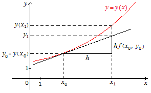
![]()
if
h is
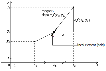
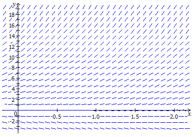
sufficiently small (small = close to 0, not close to minus infinity). See Fig.
1.1. The oblique line in this picture is the tangent of the graph of
y =
g(x)
at the point
x =
a. The
value of the function at
a +
h is
estimated by the value of the tangent line at that point. Approximation [1.1] is
called the linear or tangent-line approximation.
|
|
Fig. 1.1
Approximation:
|
Euler Method
We're considering the
IVP of the general form:
![]()
where
x0
and
y0
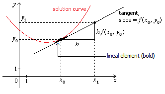
are known or given constants. Look at Fig. 1.2. Since
y0
=
y(x0),
we get the point (x0,
y0),
which is on the curve of the exact solution. We don’t know the exact value of
y at any
other point
x. So at
the next point
x1
a distance of
h > 0 to
the right of
x0
we use the linear approximation (LA) and the exact value (EV)
y0
=
y(x0)
to approximate the EV
y(x1)
by the approximate value (AV)
y1:
y1
=
y0
+
hy'(x0,
y0)
=
y0
+
h
f (x0,
y0).
At the next point x2 a distance of h to the right of x1, we use the LA and the AV y1, because we don’t have the
|
|
Fig. 1.2
y0
=
y(x0),
y1
=
y0
+
h
f
(x0,
y0),
in this case,
y1
<
y(x1).
|
EV
y2
=
y1
+
hy'(x1,
y1)
=
y1
+
h
f (x1,
y1).
Similarly, at
the next
point
x3
a distance of
h to the
right of
x2,
we use the LA and the AV
y2,
because we don’t have the EV
y(x2),
to approximate the EV
y(x3)
by the AV
y3.
And so on.
Note that
y1
isn't the EV of the solution
y at
x1;
it's an AP. The EV of course is denoted
y(x1).
In general,
yn
is the AV and
y(xn)
is the EV of the solution
y at
xn,
n = 1, 2, .
. .
A Particular Case
We illustrate the
Euler method in a particular case, the case of the IVP:
![]()
Because the general
solution of
y' =
x +
y is
y(x)
=
Cex
-
x - 1, we
have:
2 =
y(0) =
Ce0
- 0 - 1 =
C - 1,
C = 3.
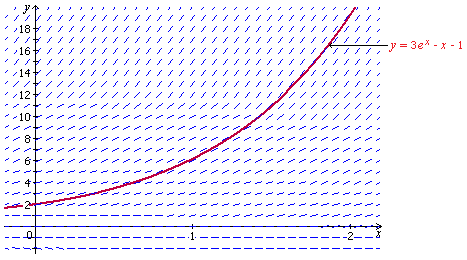
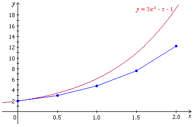
So the exact solution
of our IVP [1.2] is
y = 3ex
-
x - 1,
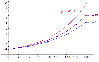
whose graph is sketched in Fig. 1.3 together with the DF of the DE in the IVP
[1.2]. In this section when we say “solution” without the qualifier “exact” or
“approximate”,
|
|
Fig. 1.3
The DF And The
Exact Solution Of [1.3].
|
it's understood to
mean the exact solution.
In the calculations
below, we pretend that we don't know that the exact solution of the IVP [1.3] is
y = 3ex
-
x - 1. Let
f
(x,
y) =
y
' =
x +
y. Because
the value of the solution at
x = 0 is
given or known (here it's
y = 2), we
employ the point
x0
= 0 as the starting point from which we go to the right to do the approximation.
See Fig. 1.3. We'll find the Euler approximate values of the solution at the
points:
x1
=
x0
+ 0.5 = 0 + 0.5 = 0.5,
x2
=
x1
+ 0.5 = 0.5 + 0.5 = 1,
x3
=
x2
+ 0.5 = 1 + 0.5 = 1.5, and
x4
=
x3
+ 0.5 = 1.5 + 0.5 = 2.
These points are
equally spaced by a horizontal distance of
h = 0.5
x-unit.
This distance is the size of the step that we make in travelling horizontally to
the right, and consequently is called the
step size
of
the approximation.
Let
y0
be the exact value (EV) of the solution curve
y =
y(x)
at
x0
= 0, so that
y0
=
y(x0)
=
y(0) = 2.
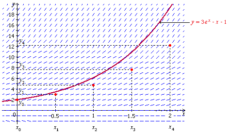
Refer to Fig. 1.4. We plot the point (x0,
y0)
= (0, 2) in Fig. 1.4. By the LA we have:
y1
=
y0
+
hf
(x0,
y0)
= 2 + (0.5)
f
(0, 2) = 2 +
(0.5)(0 + 2) = 3,
y2
=
y1
+
hf
(x1,
y1)
= 3 + (0.5)
f
(0.5, 3) = 3 +
(0.5)(0.5 + 3) = 4.75,
y3
=
y2
+
hf
(x2,
y2)
= 4.75 + (0.5)
f
(1, 4.75) =
4.75 + (0.5)(1 + 4.75) = 7.63,
y4
=
y3
+
hf
(x3,
y3)
= 7.63 + (0.5)
f
(1.5, 7.63) =
7.63 + (0.5)(1.5 + 7.63) = 12.19.
We plot the points (x1,
y1)
= (0.5, 3), (x2,
y2)
= (1, 4.75), (x3,
y3)
= (1.5, 7.63), and (x4,
y4)
= (2, 12.19) in Fig. 1.4.
Note that in
calculating
y1,
of course we use the previous point (x0,
y0),
which is a point on the exact solution. But in calculating
y2,
we don't know the previous point (x1,
y(x1))
on the exact solution to use, otherwise we wouldn't
|
|
Fig. 1.4
Euler
Approximations. |
waste time determining
the AV
y1
of
y(x1).
So we use the point (x1,
y1),
and we utilize the lineal element of the DF that passes thru that point as an
approximation of the solution curve near that point. Similarly for
y3
and
y4.
Remark that in the
computations of
yi
=
yi-1
+
h
f
(xi-1,
yi-1),
which is the Euler AV of
y(xi)
at
xi,
the point
xi
itself doesn't appear in the formula, which could mean that it wouldn't play a
role in computing the AV of the function
y at it,
which in turn doesn't seem to be right. However it does play a role, by the
presence of
h, which is
the distance from its previous point
xi-1
to it.
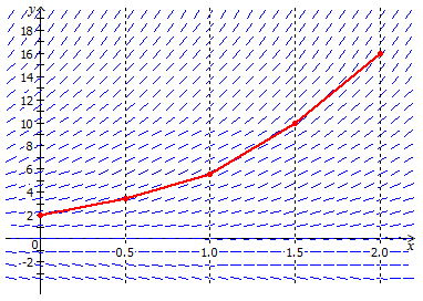
Now let's join
consecutive points by line segments, as done in Fig. 1.5. By Fig. 1.5 we're now
assured that the Euler method applied on the solution of an IVP indeed produces
an approximation of that solution, at least for a number of small steps. The set
of the values (0, 2), (0.5, 3), ..., (2, 12.19) is the
Euler
approximate numerical solution
of
the IVP [1.2]. The polygon obtained by joining these points consecutively by
line segments, colored blue in Fig. 1.5, is the
graph of the Euler approximation.
|
|
Fig. 1.5
The sequence
of line segments joining the plotted points consecutively is the Euler
Approximation. |
Better Approximations
Let's reduce the step
size from
h = 0.5 to
h = 0.25.
As evidenced in Fig. 1.6, this smaller step size provides a better approximation
than do larger ones. However reducing the step size increases the number of
steps and
|
|
Fig. 1.6
A smaller step size such as h = 0.25 provides a better approximation than does a larger one
such as
h =
0.5. |
thus the number of
points
x where to
calculate the approximations and consequently the number of calculations and
hence the number of roundings. However, even though the number of roundings
increases, generally a smaller step size still offers a better approximation
than a larger one does.
The reason for the
better approximation is as follows. In Fig. 1.6, the solid blue ellipse above
x = 0.50
actually consists of 2 points. One point is on the curve for
h = 0.50
and the other on that for
h = 0.25.
At
x = 0.50,
using
h = 0.50
you make 1 action of approximation, at
x = 0.50,
while using
h = 0.25
you make 2 actions, one at
x = 0.25
and the other at
x = 0.50
(if, eg, you use
h = 0.1,
then you make 5 actions, one at each of
x = 0.10,
0.20, . . ., 0.50). At
x = 1.00,
using
h = 0.50
you make 2 actions, while using
h = 0.25
you make 4 actions (if, eg, you use
h = 0.1,
then you make 10 actions), etc. At any point
x common to
2 or more step sizes, a smaller step size makes more actions of approximation
than a larger one does, and therefore provides a better approximation at that
point.
Return To Top Of Page
Go To Problems & Solutions
|
2. Euler Method - General Case |
Observe
that in
Fig. 1.5
the slope of the exact solution curve at the initial point (x0,
y0)
= (0, 2) is of course also the slope of the lineal element of the direction
field at that point.
In general, for the first-order IVP:
![]()
the aim of the Euler method is to determine
AVs
of the solution of this IVP at equally-spaced points:
x1
=
x0
+
h,
x2
=
x1
+
h,
=
x0
+ 2h,
. . .,
xn
=
xn-1
+
h
=
x0
+
nh,
where
h
is the constant distance between consecutive points and is called the
step size.
According to the DE in [2.1], the slope of its DF at (x0,
y0)
is
f
(x0,
y0).
So, by the LA, the
AV
y1
at
x1
is:
y1
=
y0
+
h
f
(x0,
y0),
as shown in Fig. 2.1. Similarly, the slope of the DF at (x1,
y1)
is
f
(x1,
y1),
and the AV
y2
at
x2
is:
y2
=
y1
+
h
f
(x1,
y1),
as shown in Fig. 2.2. In general, the
AV
yn
at
xn
is:
yn
=
yn-1
+
h
f
(xn-1,
yn-1),
for
n
= 1, 2, . . .
Fig. 2.1
y1
=
y0
+
hf
(x0,
y0).
|
|
Fig. 2.2
y2 = y1 + hf (x1, y1). |
Remark 2.1 – On Notations And Terminology
a.
The notation
yn
doesn't denote the
EV
of the solution at
xn,
it denotes an
AV.
The EV
of course is denoted by
y(xn),
the functional notation, as we all are already familiar with. Of course the
Euler method doesn't give the
exact solution of an
IVP. It produces approximations. However by reducing the step size we get
successively
better approximations
of the exact solution.
b.
Notice the distinction between the terminologies “method” and “approximation”:
the Euler method is a method
that produces
approximations called, of course, the Euler approximations.
Example 2.1
Consider the IVP:
![]()
a.
Use the Euler method with step size
h = 0.2 and
10 steps to calculate the AVs
y1,
y2,
. . .,
y10
of its solution.
Round your answers to
2 decimal places. Construct a table to organize these approximations.
b.
Plot these values and join the plotted points consecutively by line segments.
Solution
a.
x0
= 0,
y0
= 2,
h = 0.2,
f
(x,
y) =
x +
y,
xn
=
xn-1
+
h =
xn-1
+ 0.2,
n = 1, 2, .
. ., 10,
yn
=
yn-1
+
hf
(xn-1,
yn-1)
=
yn-1
+ (0.2)(xn-1
+
yn-1),
n = 1, 2, .
. ., 10,
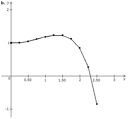
b.
The plot is depicted in Fig. 2.3.
|
|
Fig. 2.3
The sequence
of line segments joining the plotted points consecutively is the Euler
Approximation Of Example 2.1. |
EOS
Remark 2.2 - On Example 2.1
A step size generates
exactly 1 AV at any approximation point. We say that
x is an
approximation point if it’s a point where the approximation is performed. In
Example 2.1, the approximation points are
x1
= 0.2,
x2
= 0.4, etc.
Using Computers
As seen
earlier, for smaller and smaller step sizes, we get better and better
approximations. In Example 2.1, given that the number of steps is 10, there are
10 values to calculate, and
x10
= 2. Suppose we consider the step size
h
= 0.1. If we wish to reach
x
= 2, there would be (2 - 0)/0.1 = 20 values to calculate, and 2 =
x20.
In general, given an
x-range
on which to perform the approximation, of course for smaller and smaller step
sizes, the approximation becomes better and better, but
the amount of calculations becomes more and more considerable, so we should
program a computer or use a computer program to carry out these calculations.
Example 2.2 – Using A Computer For Calculations
For the IVP of Example
2.1, which is
y' =
x +
y,
y(0) = 2,
use a computer to compute the Euler estimates with 5 decimal places of
y(1) and
y(1.5) for
the 10 step sizes
h = 0.5,
0.25, 0.1, 0.05, 0.025, 0.01, 0.005, 0.0025, 0.001, and 0.0005, and construct a
table of these estimates.
Notes
a.
Each step size
h is such
that
x = 1 and
x = 1.5 are
among the
xn's.
For any step size
h,
y(1) and
y(1.5) are
estimated by
ym
and
yk
respectively for some positive integers
m and
k, where
m <
k and both
depend on
h.
b.
Even though the
question asks to find estimates of only
y(1) and
y(1.5), if
we do the computations by hand then, for this example, for each step size we
would still have to compute all the
yn's
for
n = 1, 2, .
. .,
m, where
m is such
that
xm
= 1.5, because to calculate
yn
we need to know
yn-1,
for
n = 1, 2,
...,
m. For
h = 0.0005,
there are (1.5 - 0)/0.0005 = 3000
y-values to
compute, each computation consists, as seen in the solution of Example 2.1, of 2
additions and 1 multiplication, for a total of 3 x 3,000 = 9,000 arithmetic
operations. That's a lot! And that's for just 1 step size, although all other
step sizes are larger and thus each require fewer computations. Computers
therefore are absolutely welcome.
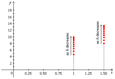
c.
If we plot the points resulting from the approximations, then we expect
something that looks similar to Fig.
2.4, provided that all the
AVs are less than the EVs.
|
|
Fig. 2.4
If the points
of Example 2.2 are plotted, they would look similar to this picture,
provided that all
the
AVs are less than the EVs. |
Solution
|
|
Fig.
2.5
|
EOS
Remarks 2.3 - On Example 2.2
a.
A step size generates exactly 1 AV at
x = 1 and
exactly 1 AV at
x = 1.5.
b.
After constructing
the table in Fig. 2.5, we realize that our plotted points in Fig. 2.4 are a
little too high. But that's ok, since the set of those points is, as we said,
similar to, not exactly like, the real thing.
c.
In Fig. 2.5, the Euler estimates appear to approach limits, which must be
the true values of
y(1) and
y(1.5) of
the exact solution of the IVP respectively.
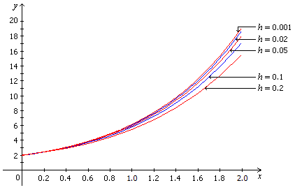
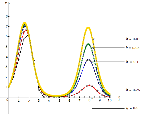
Example 2.3 – Using A Computer For Sketching
For the IVP of Example
2.1, which is
y' =
x +
y,
y(0) = 2,
use a computer to sketch the graphs of the Euler approximations of the solution
for the 5 step sizes
h = 0.2,
0.1, 0.05, 0.02, and 0.001 for the interval [0, 2].
Solution
|
|
Fig. 2.6
Graphs Of The Euler Approximations Of
Example 2.3. |
EOS
Remarks 2.4 - On Example 2.3
a.
Each step size
h must be
such that the last point
xn
equals 2.
b.
In Fig. 2.6, each
x-interval
represents 0.2 unit. So, for
h = 0.2,
each interval contains 1 step excluding its left endpoint, thus 1 point where to
do the approximation; for
h = 0.1,
each interval contains 0.2/0.1 = 2 steps excluding its left endpoint, thus 2
points where to do the approximations; for
h = 0.001,
each interval contains 0.2/0.001 = 200 steps excluding its left endpoint, thus
200 points where to do the approximations. Each graph is actually a sequence of
consecutively-joint line segments. As
h gets
smaller and smaller, the line segments in this example become shorter and
shorter because their count in each interval of fixed length 0.2 unit gets
larger and larger, hence the graphs look more and more like smooth curves.
c.
As
h
approaches 0, the graphs of the Euler approximations seem to approach a limit,
which must be the graph of the exact solution of the IVP.
Determining A Formula For
yn
And Determining The Number Of Steps
Example 2.4 - Formula For
yn
And Number Of Steps
Consider the IVP:
![]()
Use the Euler method
with step sizes
h = 0.1,
0.01, 0.001, 0.0001, and 0.00001 to estimate
y(2),
without utilizing a computer. Do the AVs seem to approach a value? If yes, what
value? Note: The exact solution is
y =
ex.
Hint: Find a formula for
yn
in terms of
y0
(=
y(0)),
h, and
n, and for
each step size determine
n such that
yn
estimates
y(2).
Note
For each step size,
the
x-points
are
x0
= 0,
x1,
x2,
. . .,
xn
= 2, and
n is such
that
yn
is the AV of
y(2) for
that step size. Remark that the subscript starts from 0, not 1, so there are
n
consecutive intervals: [x0,
x1],
[x1,
x2],
. . ., [xn-1,
xn],
and thus
n steps and
there would be
n values to
calculate. The length of each interval is the step size
h. As a
consequence,
hn =
xn
–
x0
= 2 – 0 = 2. Hence
n = 2/h.
If for each step size we calculate all the values
y1,
y2,
. . .,
yn,
there would be 2/0.1 + 2/0.01 + 2/0.001 + 2/0.0001 + 2/0.00001 = 222,220 values
in total to calculate. And we're not allowed to utilize a computer. Because it's
impractical to calculate all the 222,220 values by hand, especially in a test or
exam, we have to determine a formula for
yn,
which will be in terms of the known quantities
y0
and
h and the
readily-computed quantity
n, as
demonstrated in the solution. Then for each step size, we'll have to compute
only 1 value, namely
yn.
Solution
We have
x0
= 0,
y0
= 1, and
f
(x,
y) =
y. So:
yn = yn-1 + h f (xn-1, yn-1)= yn-1 + hyn-1 = (1 + h)yn-1 = (1 + h)(yn-2 + hyn-2) = (1 + h)(1 + h)yn-2 = (1 + h)2yn-2
= (1 +
h)2(yn-3
+
hyn-3)
= (1 +
h)3yn-3
= . . . = (1 +
h)nyn-n
= (1 +
h)ny0.
= (1 +
h)n(1)
= (1 +
h)n.
For each step size
h the
number of steps is
n = (2 -
0)/h
= 2/h
and
yn
estimates
y(2).
Yes, the AVs seem to
approach a value, which must be the EV
y(2) =
e2,
which is approximately 7.38906.
EOS
Remark 2.5 - Number Of Step Sizes And Number Of Approximation Points
In Example 2.4, a step size generates exactly 1 AV at x = 2. Similar remarks are also made in Remarks 2.2 and 2.3. So to avoid confusion about the number of step sizes and the number of approximation points, we keep this in mind: a step size generates exactly 1 AV at any approximation point. For the definition of approximation point, see Remark 2.2.
Return To Top Of Page
Go To Problems & Solutions
|
3. Error In The Euler Method |
We saw earlier under
the heading
Euler Method in this section that the exact solution of the IVP:
![]()
is
y = 3ex
-
x – 1. The
Euler AVs of the solution for the step size
h = 0.5 at
the points
x1
= 0.5,
x2
= 1,
x3
= 1.5, and
x4
= 2 were calculated to be
y1
= 3,
y2
= 4.75,
y3
= 7.63, and
y4
= 12.19 respectively. Because the exact solution for this particular IVP is
known, we can compare the AVs to the EVs. The
error of the Euler method is of
course the difference between the AV and the EV. The
absolute error is the absolute value
of the error. So:
error = AV - EV,
absolute error = |error| =
|AV
- EV|.
The AVs are estimates
of the corresponding EVs. If an estimate is less than the EV, the error is
negative, and we say that the estimate is an
under-estimate
(because it's under the EV). If an estimate is greater than the EV, the error is
positive, and we say that the estimate is an
over-estimate
(because it's over the EV).
The table in Fig. 3.1
displays the EVs, the Euler AVs, the errors, and the absolute errors for the
solution of [3.1] for the step size
h = 0.5 at
the indicated points
x. As the
exact solution itself involves the exponential function,
|
|
Fig. 3.1
Error In Euler
Method. |
|
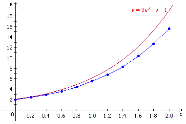
|
Fig. 3.2
The sequence of line segments joining the plotted
points consecutively is the Euler
Approximation. |
we have to settle with
the decimal approximations of the EVs. Fig. 3.2 displays the exact-solution
curve and the approximate-solution curve. Notice that as seen in Figs. 3.1 and
3.2, the absolute error increases as
x moves to
the right away from
x0,
which is 0 in this case. Algebraically the error decreases, as a negative
quantity that gets larger in size decreases, algebraically speaking. Saying that
the error decreases would be misleading in its everyday sense. So to avoid this
problem we employ the absolute error.
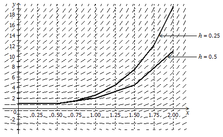
Fig. 1.6 is re-produced as Fig. 3.3. Clearly as the step size is
halved from
h = 0.5 to
h = 0.25,
the absolute error (here at the points
x = 0.50,
1.00, 1.50, and 2.00) is roughly halved too.
|
|
Fig. 3.3
If the step size is halved then the absolute
error is roughly halved too. |
In general, the absolute error in the Euler method possesses these properties:
1. For any 1 step size
h,
when
x
increases away from
x0,
the absolute error tends to increase as well.
2. At
any 1 point
x,
when
h
decreases, the absolute error tends to be proportional to
h.
For example, decreasing
h
by half decreases the absolute error by approximately half as well.
These properties are studied in depth in courses on differential equations and
courses on numerical analysis (numerical analysis is now sometimes also called
scientific computations).
Return To Top Of Page
Go To Problems & Solutions
|
4. Graphing Euler Approximation Using Only
The Direction Field |
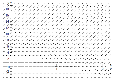
Suppose that we're given a DF, as displayed in Fig. 4.1, and that we're asked to sketch the graph of the Euler approximation of the exact solution curve that passes thru the point (0, 2), with step size 0.5 and 4 steps. This
|
|
Fig. 4.1
A given DF. |
is an IVP, with
y(0) = 2,
but we have only a DF instead of an explicit DE of the form
y
' =
f
(x,
y). So of
course we cannot use the formula
yn
=
yn-1
+
h
f
(xn-1,
yn-1).
We have to utilize the DF itself.
Recall that the
formula
yn
=
yn-1
+
hf
(xn-1,
yn-1)
is the tangent-line approximation, as seen in
Fig. 1.2 for
n = 1,
re-produced below for convenience as Fig. 4.2. We draw the tangent line of the
curve at the point (xn-1,
yn-1),
this tangent intersects the vertical line
x =
xn
at a point, the
y-coordinate
of this point is
yn,
this point is the desired point (xn,
yn).
Let's employ a similar process for a DF. Refer to Fig. 4.3, which is
Fig. 2.2 re-produced here for
|
|
Fig. 4.2
y0
=
y(x0),
y1
=
y0
+
h
f
(x0,
y0),
in this case,
y1
<
y(x1). |
|
|
Fig. 4.3
y2
=
y1
+
h
f
(x1,
y1). |
convenience. For
example, at the point (x1,
y1),
we draw a tangent line from that point that's parallel to the lineal element at
that point, or parallel to the lineal element nearest to that point. That
tangent intersects the vertical line
x =
x2
at the point (x2,
y2).
|
|
Fig. 4.4
Graph Of Euler
Approximation. |
Return To Top Of Page
Go To Problems & Solutions
|
5. A Thought On Numerical Methods |
The idea behind the
numerical method for first-order ordinary differential equations is to
approximate the numerical
y-values
of a solution for a given or chosen finite discrete sequence of
x-values:
x1,
x2,
. . .,
xn,
equally spaced.
We start at an initial point (x0,
y0)
on a solution curve and then calculate the
y-values
y1,
y2,
. . .,
yn
that approximate the actual
y-values
y(x1),
y(x2),
. . .,
y(xn)
respectively. The points (x1,
y1),
(x2,
y2),
. . . , (xn,
yn)
represent the approximations of the actual points (x1,
y(x1)),
(x2,
y(x2)),
. . . , (xn,
y(xn))
respectively. The actual points are the ones that actually lie on the graph of
the solution
y(x),
which is usually unknown. The value
y0
is the actual value of the solution at
x0.
So what we do is to determine numerically an approximation of the solution that
passes thru the point (x0,
y0).
Graphically, by joining the consecutive points (x0,
y0),
(x1,
y1),
. . . , (xn,
yn)
by line segments, we obtain a polygon, which hopefully has qualitative
characteristics that are close to those of an actual solution curve.
The Euler method is simply one of many different numerical methods in which a
solution of a DE can be approximated. Other numerical methods, notably the
fourth order Runge-Kutta method, provide
significantly greater accuracy than the Euler method does. However the Euler
method is the place to start the learning of numerical methods for DEs.
Problems & Solutions
|
1.
Consider the IVP:
a.
Use the Euler method with step size
h = 0.25
and 10 steps to calculate the AVs
y1,
y2,
. . .,
y10
of its solution.
Round your answers to
2 decimal places. Construct a table to organize these approximations.
b.
Plot these values and join the plotted points consecutively by line segments.
Solution
a.
x0
= 0,
y0
= 1,
h = 0.25,
f
(x,
y) =
xy -
x2,
xn
=
xn-1
+
h =
xn-1
+ 0.25,
n = 1, 2, .
. ., 5,

2.
Use a computer to compute the Euler estimates with 5 decimal places of
y(2.5) and
y(3) for
the 10 step sizes
h = 0.5,
0.25, 0.1, 0.05, 0.025, 0.01, 0.005, 0.0025, 0.001, and 0.0005, and construct a
table of these
estimates, for this
IVP:

Solution
3.
Consider the IVP:
Solution
4.
Consider the IVP:
![]()
a.
Verify that its exact solution is
y = (1.8)e2x.
b.
Use the Euler method with each of the following step sizes to estimate the value
of
y(1.5)
without utilizing a
computer:
h = 0.1,
0.05, 0.025, 0.0125, 0.00625, and 0.003125. Note that each step size from the
second on
is half of the
previous one. Do the AVs appear to tend to a value? If yes, what value?
Hint: Find a formula
for
yn
in terms of
y0
= 1.8,
h, and
n. For each
step size, determine
n such that
yn
is the AV of
y(1.5).
c.
State which estimates are over-estimates and which are under-estimates.
d.
Find the error and the absolute error in the Euler method in part b for each
step size. Each time the step size
is cut in half, what
happens to the absolute error?
a.
If
y = (1.8)e2x
then
y
' = 2(1.8)e2x
= 2y
and
y(0) =
(1.8)e0
= 1.8. So
y = (1.8)e2x
indeed is the exact solution of
the given IVP.
b.
We have
x0
= 0,
y0
= 1.8, and
f
(x,
y) = 2y.
So:
yn
=
yn-1
+
h
f
(xn-1,
yn-1)
=
yn-1
+
h(2yn-1)
= (1 + 2h)yn-1
= (1 + 2h)(yn-2
+
h(2yn-2))
= (1 + 2h)2yn-2
=(1
+ 2h)2(yn-3
+
h(2yn-3))
= (1 + 2h)3yn-3
= . . . = (1 + 2h)nyn-n
= (1 + 2h)ny0
= (1.8)(1 + 2h)n.
For each step size
h the
number of steps is (1.5 - 0)/h
= 1.5/h.

Yes, the AVs appear to
tend to a value, which must be the EV
y(1.5) =
(1.8)e2(1.5)
= (1.8)e3,
which is
approximately
36.15397.
c.
Because the EV is approximately 36.15397, all the estimates are under-estimates.
There's no
over-estimate.
Each time the step
size is cut in half, the absolute error is roughly cut in half too.
5.
For the IVP:
![]()
show that, when using
the Euler method with step size
h, the
estimate
yn
of
y(xn)
is given by the formula:
yn
= (nh)2
+ (2 -
h)nh
+ 2.
Note that
xn-1
and
yn-1
don't appear in this formula.
We have
x0
= 1,
y0
= 2, and
f
(x,
y) = 2x.
So:

Note
We use the formula:
6.
A DF for a DE is displayed below. Sketch the graphs of 2 Euler approximations of
the solution curve that
passes thru the point
(0, 1). Use step sizes
h
= 0.5 and
h
= 0.25 and go till
x
= 2.
7. It can be shown that for the IVP y' = f (x, y), y(x0) = y0, as the step size h decreases toward 0, then the
Euler approximations converge to the exact solution, provided f satisfies some conditions. This problem gives
an example to illustrate
this property of the convergence of the Euler method. Consider this IVP:
Solution
Return To Top Of Page
Return To Contents